Digital Filter Design With Matlab
Matlab FILTER instruction filters discrete signal with specified FIR/IIR(numerator B and denominator A in Direct Form II form) filter coefficients. Both filter and filter2 (used for 2D filtering) instructions are available in student edition. Type "help filter" for more information.
Other filter implementation instructions include:
cconv - Modulo-N circular convolution
convmtx - Convolution matrix
filtfilt - Zero-phase digital filtering
sosfilt - Second-order (biquadratic) IIR digital filtering
Digital Filters
FIR
cfirpm - Complex and nonlinear-phase FIRfir1 - Window-based finite impulse response
fir2 - Frequency sampling-based finite impulse response
firls - Least square linear-phase FIR
firpm - Parks-McClellan optimal FIR
intfilt - Interpolation FIR
kaiserord - Kaiser window FIR estimation parameters
sgolay - Savitzky-Golay
IIR
butter - Butterworthcheby1 - Chebyshev Type I (passband ripple)
cheby2 - Chebyshev Type II (stopband ripple)
ellip - Elliptic
maxflat - Generalized digital Butterworth
yulewalk - Recursive digital
Mathoworks Example
Cascade a lowpass filter and a highpass filter to produce a bandpass filter:
[b1,a1]=butter(8,0.6); % Lowpass
[b2,a2]=butter(8,0.4,'high'); % Highpass
H1=dfilt.df2t(b1,a1);
H2=dfilt.df2t(b2,a2);
Hcas=dfilt.cascade(H1,H2); % Bandpass-passband .4-.6
Conversion (Analog to Digital)
bilinear - Bilinear transformation
impinvar - Impulse invariance
Analog Filters
Design
butter - Butterworth
cheby1 - Chebyshev Type I (passband ripple)
cheby2 - Chebyshev Type II (stopband ripple)
besself - Bessel analog
ellip - Elliptic
Transformation
lp2bp - Lowpass analog filters to bandpass
lp2bs - Lowpass analog filters to bandstop
lp2hp - Lowpass analog filters to highpass
lp2lp - Change cutoff frequency for lowpass filter
For information visit: mathworks.com/access/helpdesk/help/toolbox/signal/f9-131178c.html
Bilinear Transform
This method is an approximation technique that transforms systems transfer functions from discrete z-domain to continuous s-domain:
For more information visit: en.wikipedia.org/wiki/Bilinear_transform
Hilbert Transform
Hilbert transform is the process of multiplying a Fourier transformed function by -jsgn(w)-sgn(w) is negative for w > 0, zero at w = 0 and positive for w < 0
Hilbert transform shifts the phase of the:
- negative frequency components by +90° (p/2 radians)
- positive frequency components by -90° (p/2 radians)
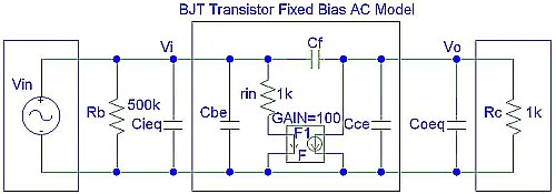
Miller Effect

|
stray capacitance.sch Size : 0.005 Kb Type : sch |
Equivalent Output Capacitance
Current from output to ground:
Vo/Zoeq = -(Vi-Vo)/Zf
Zoeq = -Vo*Zf/(Vi-Vo)
Assume: Vo = Av*Vi (Av = -Rc/(rin/Hfe))
Zoeq = -Zf*Av/(1-Av)
Zoeq = Zf/(1-1/Av)
Coeq = Cf*(1+1/|Av|) for Av < 0
en.wikipedia.org/wiki/Miller_effect